Physics-Informed Neural Networks: Constraints and Validation

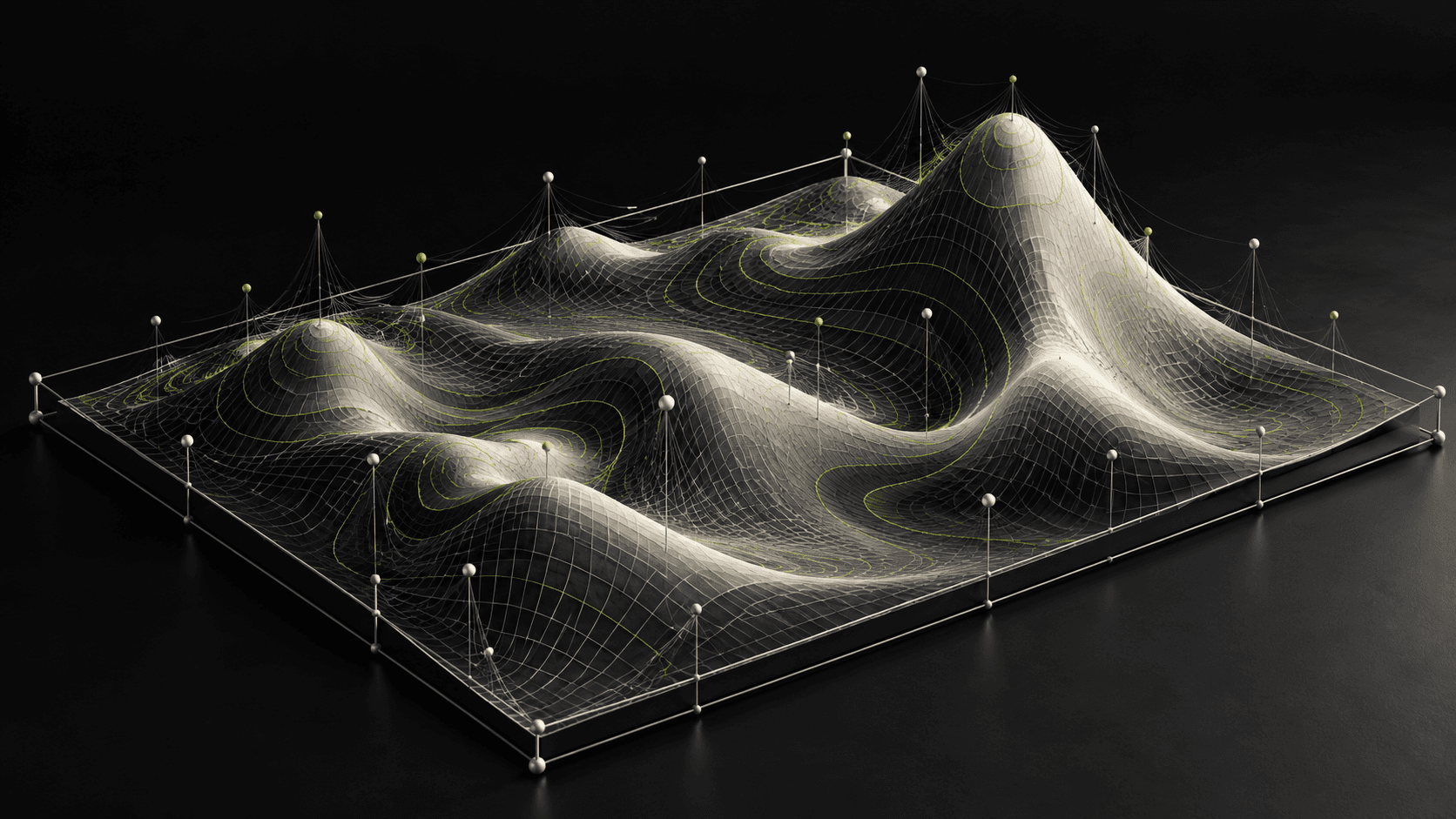
In scientific and engineering problems, observations are often limited while some of the governing structure is already known. A temperature field may satisfy a diffusion equation. A mechanical system may obey a balance law. A useful model should make sense of the measurements without discarding that structure.

Physics-informed neural networks, usually called PINNs, incorporate physical constraints into the learning problem. They do not make a network a simulator by definition, and adding an equation to a loss function does not guarantee a physically valid solution.

What goes into a PINN objective?

A network can represent an unknown field as a function of space and time. Automatic differentiation computes derivatives of that representation. A training objective can then combine disagreement with observed data, a governing-equation residual at sampled collocation points, and violations of initial or boundary conditions.

A simplified description is: total loss equals weighted data error plus weighted equation residual plus weighted condition error. The weights matter because the terms can have very different scales and gradients. Automatic differentiation describes derivatives of the chosen network; it does not certify that the learned field solves the physical problem.

Some methods enforce selected constraints through the architecture or output parameterization instead of penalizing violations. That can provide stronger satisfaction of those specific constraints. It still leaves questions about the remaining equations, numerical approximation, observations, and domain assumptions.

Why a low training loss can mislead

Residuals are checked at selected points. A model can perform poorly between them, near a boundary, or at an under-resolved transition. Incorrect units, poor nondimensionalization, incompatible loss scales, and optimization difficulties can all interfere with learning.

The NeurIPS study of PINN failure modes shows that even modestly more challenging physical problems can create difficult optimization landscapes. Its analysis is a useful warning against assuming that adequate model expressivity makes training reliable. Reported improvements from a particular training method remain specific to the studied problems.

Validation should therefore include held-out observations, dense residual checks where feasible, boundary-condition error, physically relevant quantities, and comparison with a trusted numerical solution or analytical case. A visually smooth field is not enough.

Recent work: the constraints themselves need scrutiny

The 2026 Communications Physics paper Enforcing hidden physics in physics-informed neural networks studies irreversibility-related constraints that conventional training can miss. Its contribution is a concrete reminder that the written differential equation and the desired physically admissible behavior may not be captured adequately by a basic residual objective. The paper's benchmark improvements do not establish a universal guarantee for every PDE.

The September 2026 lecture notes on PINNs and neural operators provide a current learning resource spanning implementations and newer scientific-ML directions. They are educational notes distributed as a preprint, rather than a new benchmark proving that one method wins everywhere.

Inverse problems and neural operators

PINNs can be attractive when unknown physical parameters must be estimated alongside a field from sparse measurements. However, parameter identifiability matters: several parameter settings may fit the same observations. Extra optimization cannot recover information the measurements do not contain.

Neural operators address a related but different objective: learning mappings between functions, such as a family of input conditions and their corresponding solution fields. A conventional PINN is often optimized for a particular problem instance. The approaches can overlap, but neither label should be used as a synonym for the other.

For repeated queries across a parameter family, an operator-learning approach may be worth comparing. For a sparse inverse problem with known equations, a PINN may be a useful candidate. In either case, conventional numerical methods belong in the comparison rather than being dismissed because they are older.

What I would check before using a PINN

Write the equations, units, assumptions, and valid operating regime explicitly.
Check whether the available measurements identify the unknown parameters.
Validate on a simple analytical or numerical reference before expanding the problem.
Track each loss component and its gradients instead of only the total loss.
Compare error, robustness, training cost, and query cost against appropriate baselines.

For industrial monitoring, a meaningful first question is whether the physics model is accurate enough to constrain the observations. If operating conditions change or important effects are omitted, a strong physical penalty can reinforce the wrong assumptions. Useful scientific AI makes that boundary visible.

Sources and further reading

Research perspective. Sources checked on 20 October 2026; this article reports no new simulation or experimental result.

PINNs: Learning Under Physical Constraints